Welcome to my thesis
Thesis overview: My thesis focuses on the Fucus distichus in San Francisco Estuary, looking at both its current status and how climate change could affect it in the future. To accomplish this there were two parts to my thesis: field work and an experiment. The field work took place at four field sites in Central San Francisco Bay with monthly surveys from June 2018 to Septemeber 2019. Population data was recorded in the field and samples were taken to be processed in the lab. The mesocosm experiment manipulated carbonate chemistry and salinity levels to study its affect on the reproductive output (oogonia) of Fucus distichus.
Research Questions
- What is the distribution and abundance of F. distichus in SFE and how does the population structure change over time?
- What is the reproductive phenology of F. distichus in SFE?
- Is variation in salinity, air temperature, or pH associated with changes in abundances or reproductive effort of F. distichus populations in SFE?
- Do changes to estuarine salinity and pH influence the reproductive output of F. distichus?
Data and calculations
Data: Both raw and calculated data available here
Field data calculations: markdown with calculations
Environmental data wrangling: data wrangling and final dataset, some of the raw data sets I downloaded are too large to upload on GitHub so I removed unneeded columns
Filtering for tides: markdown. Since Fucus distichus is an intertidal species, it experiences periods of time out of the water. To address this, I filtered out water data (pH, salinity, and water temperature) when it was exposed (<1m). I did the opposite for air temperature, I filtered out data when it was underwater.
Lining up environmental data with field data: environmental data filtered between field survey dates, environmental data filtered 30 days before field survey dates, environmental data filtered 60 days before field survey dates
Mesocosm calculations:Rmarkdown
This is also the order I worked through data if you’re interested in doing something similar.
1. What is the distribution and abundance of F. distichus in SFE and how does the population structure change over time?
- Field site and bouy locations map: We conducted monthly ecological F. distichus surveys at four sites from June 2018 to September 2019. Surveys were conducted at low tide once a month and at least three weeks apart between months. When we first surveying potential field sites, we referenced iNaturalist to see where F. distichus has been found. We picked four accessible representative sites to capture the variability of Central San Francisco Estuary (SFE). Field sites were located in Central SFE along the salinity gradient at Horseshoe Bay (37.83, -122.48), Brickyard Park (37.88, -122.50), Point Chauncy (37.89, -122.45), and Paradise Cay (37.92, -122.48). Each site has a monitoring buoy relatively close to each one so that we could characterize the salinity and temperature of each site.
- Distribution of Fucus distichus in San Francisco Bay map, Rmarkdown: Distribution of F. distichus in San Francisco Estuary was determined mapping observations from iNaturalist, Josselyn and West (1985) and Whitaker et al. (2017). I downloaded 299 observations of Fucus distichus from iNaturalist (May 15, 2020). iNaturalist is a citizen science platform where users upload pictures of species with linked GPS coordinated. Only research grade observations of F. distichus in SFE on iNaturalist where downloaded. I then assessed each photo and assigned it as “attached,” “wrack,” or “unclear.” I then mapped this database in a map on R (package “leaflet”).
- Phenology analysis mixed model, visualization
- Percent cover Rmarkdown: Standard quadrat transect sampling was used. Parallel to the shore, we placed a 15m transect through the middle of a healthy F. distichus population. The transect location was consistently within 0.5m throughout the sampling period. Random points (n=10) were selected along the transect and a 0.25m^2 quadrat was used for sampling. We measured percent cover in each quadrat.
- Total, large thalli and small thaiil density Rmarkdown: Density was measured by counting the number of holdfasts in the quadrat. Individuals with holdfasts outside of the quadrat were not counted. Individuals were then assigned into one of two size classes: small with individuals less than 12cm in length and large individuals longer than 12cm in length.
- Opportunistic comparasion of 2018 versus 2019
- 2018 vs 2019 Fucus distichus bed length table, Rmarkdown: This was an opportunist comparison of F. distichus in May 2018 versus May 2019. In May 2018, I scouted Central SFE for potential field sites of F. distichus looking for dense beds of at least 10 m in length. When I found dense beds, I recorded the GPS end points of the beds and in May 2019 I revisited the same sites. I used the “measure” tool on ArcGIS online to convert GPS points into lengths along the shoreline.
2. What is the reproductive phenology of F. distichus in SFE?
- Field Methods: In the field, one specimen was randomly selected from each quadrat (n=10) for lab analysis. Samples were collected and immediately placed in sealed bags that were taken to the lab within 2 hours of collection times. Samples that were not immediately processed were placed in a dark refrigerator at a constant temperature (type, temp). Samples were processed within two weeks of collection. All samples were first inspected for and removed of epiphytes and invertebrates before proceeding.
- Reproducitve anatomy and lab methods: Reproductive tissue allocation was assessed in two ways. First, reproductive tissue allocation was calculated as a percentage of reproductive apices diagram (Graiff et al. 2017). Apices were considered reproductive with the presence of visible conceptacles. Second, reproductive tissue allocation was calculated by biomass. Reproductive apices were cut and separated from the vegetative portion of each sample. Samples were then placed in a drying oven at 17C for at least 48 hours (oven model). Dry reproductive and dry vegetative weights were then recorded to the nearest thousand decimal place on an analytical scale. We combined the density data and reproductive potential data to estimate oogonia/ow we calculated oogonia/0.25m^2 – calculated to incorporate oogonia per conceptacle, m^2 each month at each site. (conceptacle per reproductive apex, reproductive apex per adult thalli, and adult thalli per 0.25m^2 and was then square root transformed. this takes the oogonia in an individual thalli and scales it to an ecological context). These methods are based from Graiff (2017) and Pearson and Brawley (1996). I quantified reproductive potential of 3 of the 10 collected samples. These 3 samples were randomly selected. Reproductive potential is defined here as the number of oogonia within conceptacles of F. distichus. Quantifying the reproductive potential indicated how many eggs are available for release. From the 3 selected samples, I randomly selected a reproductive apex from each sample and I counted the number of conceptacles present. Then from each selected apex, I cut three conceptacles out to section with a razor blade, hydrate with water, and place it on a slide. Each slide was inspected under xmag/microscope where I counted the oogonia for each of the selected conceptacles diagram.
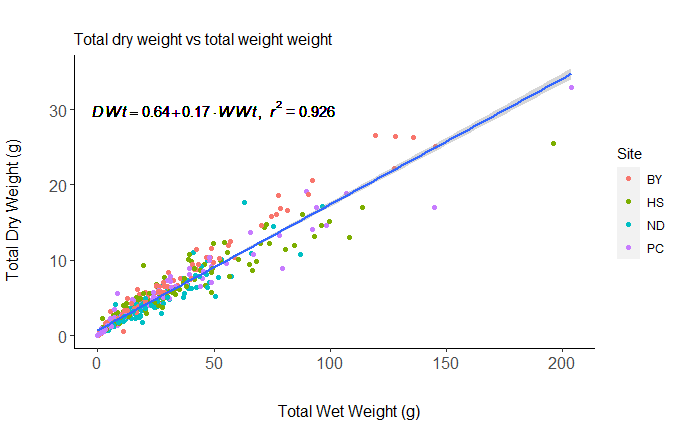
- Varifying lab methods: total dry weight vs total wet weight- graph, Rmarkdown
- Oogonia per meter: Rmarkdown
- Oogonia per thalli: Rmarkdown
- Oogonia per conceptacle: Rmarkdown
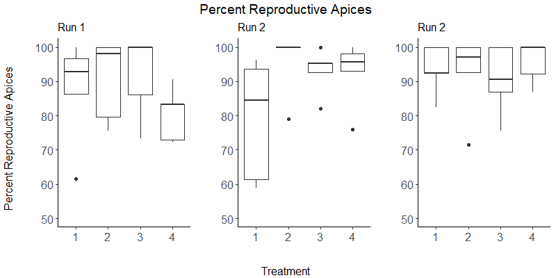
- Percent Reproductive Apices: Rmarkdown
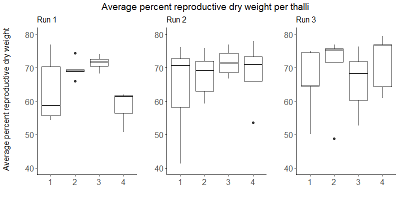
- Percent Reproductive Dry Weight: Rmarkdown
- Reproductive percent cover in field:Rmarkdown
- Reproductive dry weight vs reproductive apices: Rmarkdown
- Percent reproductive dry weight per thalli: Rmarkdown
3. Is variation in salinity, air temperature, or pH associated with changes in abundances or reproductive effort of F. distichus populations in SFE?
Environmental data graphs, table summarizing environmental conditions per site during field survey dates
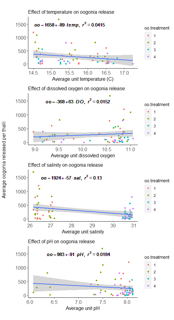
4. Do changes to estuarine salinity and pH influence the reproductive output of F. distichus?
Mesocosm Experiment: Efects of pH and salinity on oogonia released
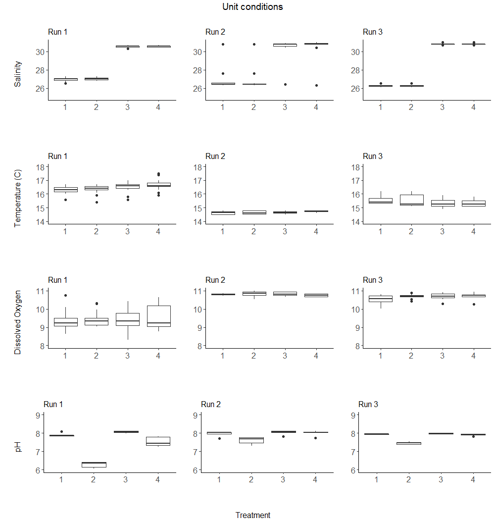
Experimental set up and design
Oogonia released under different pH and salinity conditions
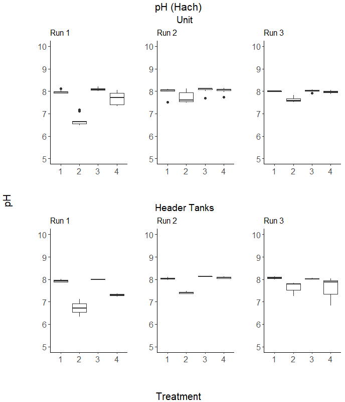
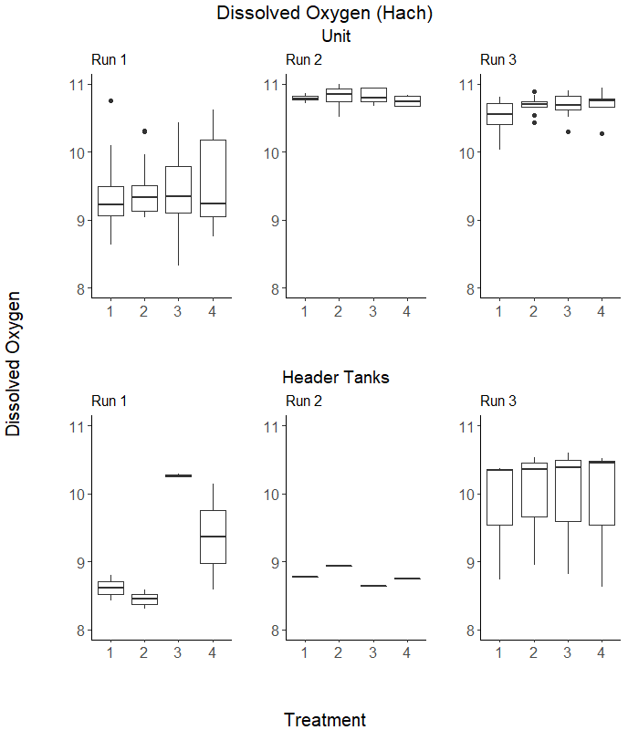
Unit conditions
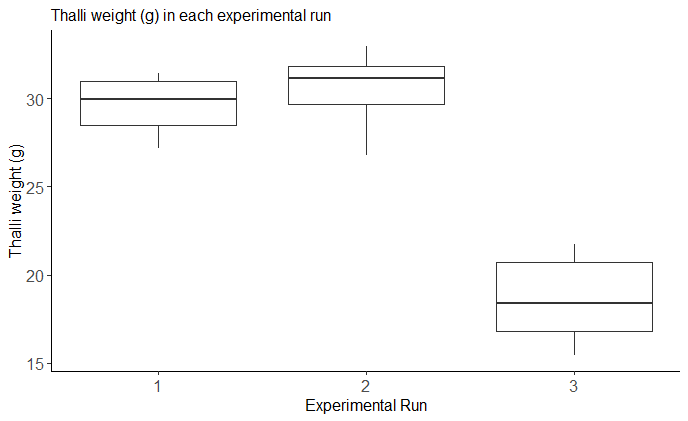
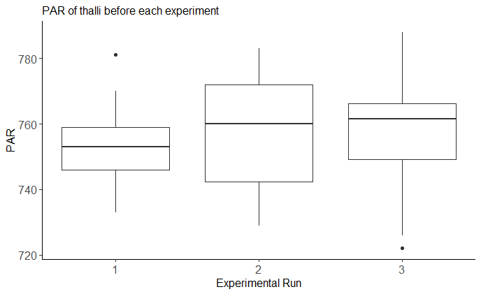
Experimental thalli
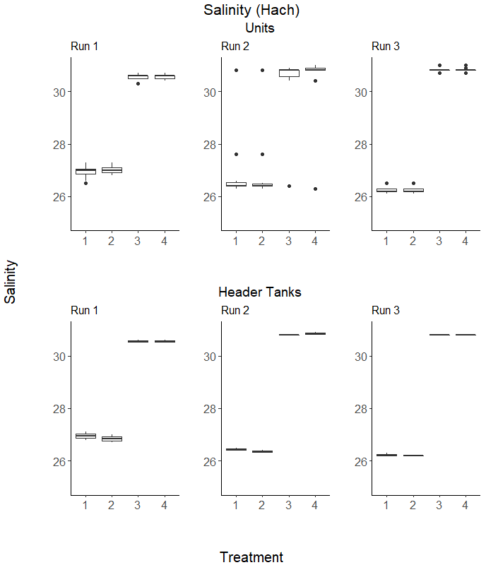
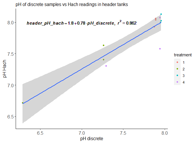
Verifying Hach readings
Discussion
**Old attempts and approaches no longer being used (double check before removing)
- Enviormental data all, salinity, pH, dissolved oxygen, water temeperature, metadata
- data set-up
- data question, revised
- analysis attempt, finding best fit, new
- air temperature data and tide filtering, ended up merging this in the other environmental variable markdowns
- Mesocosm
- Heatmap: Rmarkdown
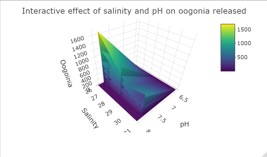
- Interactive effect of salinity and pH on oogonia release: graph with markers, graph with surface contour, Rmarkdown, potential picture for print
- AIC example